

This is a quick tutorial on how to freeze rows in Excel. I know that most of you don’t need pointers with this, but if you’re new to Excel, keep reading to get familiar with the basics.
This feature can come in handy when you have an Excel document that is so long that you need to scroll to see all the information but you want to keep the first row always visible. Or in case of sideways scrolling, make the first column sticky.
Freeze the first row and/or column
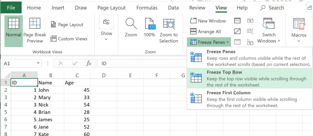
Top Row
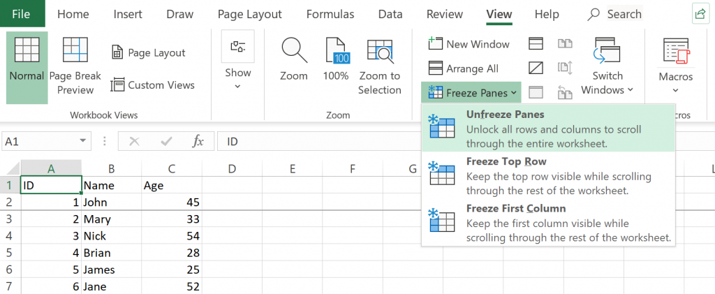
In order to freeze just the top row in Excel, you’ll need to select View > Freeze Panes > Freeze Top Row.
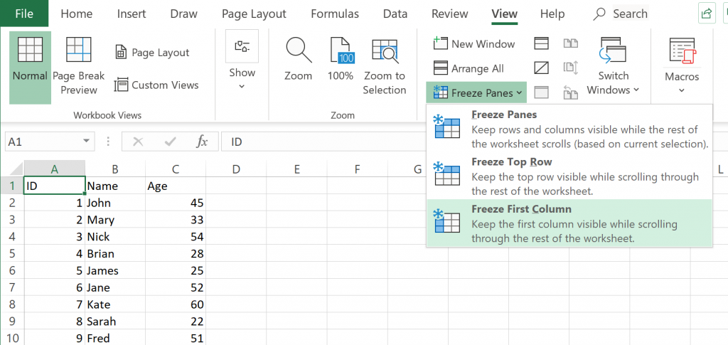
First Column
To freeze only the first column, you’ll need to select View > Freeze Panes > Freeze First Column.
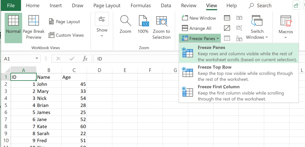
Top Row and First Column
To freeze them both, you’ll need to select View > Freeze Panes > Freeze Panes
Note: Only one of the three options can be active at a time. Meaning – if you freeze the top row and later decide that you also want to freeze the first column, you’ll need to choose “Freeze Panes” since clicking on “Freeze First Column” will unfreeze the top row.
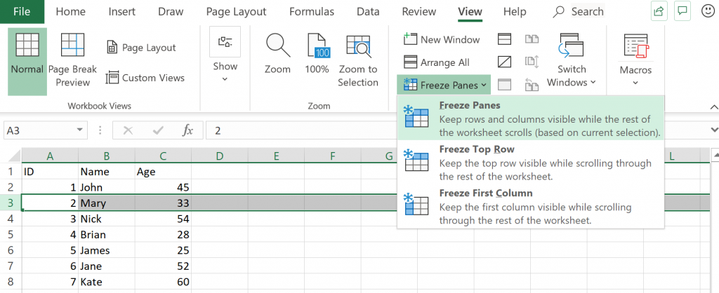
Freeze Multiple Rows
To freeze more than one row and/or column, select the first row/column that you don’t want to stay sticky. And just like before, go to View > Freeze Panes > Freeze Panes.
In the below example, both the first and second row will be frozen.
Unfreeze rows
To unfreeze, simply go to View > Freeze Panes > Unfreeze Panes
Note: Excel will automatically draw a grey line underneath the rows/columns that you have frozen to indicate what will always stay in view.