

The CONCATENATE function in Excel enables a user to join two or more cells into one. We often need to join the first and last name into a full name or street, house number and city into a full address. One of the easiest ways to complete this is using the Concatenate function. In this tutorial, we will see how to use the function to concatenate texts, cells references, function results, etc.
Formula Syntax Explanation
The syntax of the CONCATENATE function in Excel looks like:
=CONCATENATE(text1, [text2], [text3], …)
The parameters of the function are:
text1, [text2], [text3]
These are texts which we want to concatenate, separated with a comma. Only one text is mandatory, while up to 255 texts can be passed to the function. The function accepts all kinds of data, including numbers, dates, other functions, cells references, etc. As a result, the function will return a text, regardless of the input data formats.
Please note that from Excel 2016, the function CONCAT is introduced instead of the CONCATENATE function. These functions have the same syntax and almost similar results. The only difference is that the CONCAT function works with ranges, which will be explained more later. However, we will explain all the examples on the CONCATENATE function, because of the compatibility with the older Excel versions.
Basic usage of the CONCATENATE function
We will first look at the most simple example of the function, which includes joining two texts. In the example, we want to concatenate “Mike“ and “Johnson” in the cell B3 to get the full name. The formula is:
=CONCATENATE(“Mike “, “Johnson”)
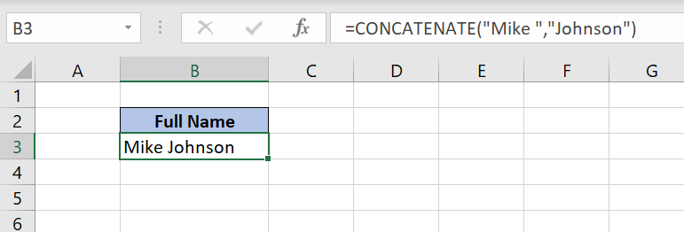
As you can see in Image 1, all the texts which we want to join, need to be put under quotations (“). As a result, we get “Mike Johnson” in cell B3.
Now we will see how to do the same concatenation, but with cell references instead of texts. In this example, the first name is in the cell B3, while the last name is in the cell C3. The result of the function is in the cell D3. The formula is:
=CONCATENATE(B3, C3)

As we can see in Image 1, values from B3 and C3 are concatenated into “MikeJohnson” in the cell D3. In this example, we need to add a space between the first and last name to make the output valid.
Concatenate cells with spaces and other symbols
In order to add a space between two cells, we need to put a space under the quotations (“ “) as a parameter of the function. The formula is:
=CONCATENATE(B3, ” “, C3)
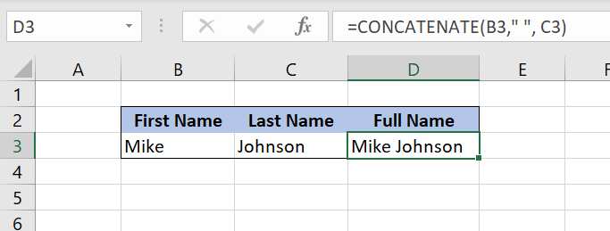
Now the output of the function in D3 is the full name with a space between the first and last name (“Mike Johnson”).
Similarly to this example, we can join two cells with a comma between. In this case, we need to put a comma instead of space. The formula looks like:
=CONCATENATE(B3, “, “, C3)

Image 4. Concatenation of two cells with a comma
The result of the function in the cell D3 is “Mike, Johnson”. Similarly to this example, we can add any separator between the two cells.
Concatenate a text and cell values
As we saw in the previous example, the CONCATENATE function can work with both cells and texts. Now we will see how to combine cells and text in the same formula. In the cell D3 we want to concatenate the text “Fullname:“ and cells B3 and C3 with a space. The formula is:
=CONCATENATE(“Fullname: “,B3,” “, C3)
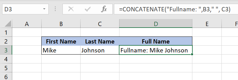
The result of the function in D3 is “Fullname: Mike Johnson”. As you can see in Image 5, the function can combine texts and cells in concatenation.
Concatenate cells with a line break
Another possible option is to concatenate cells with a line break. This is possible by using the CHAR function which takes an ASCII code and returns a special character. In our case, the ASCII code for a line break is 10. Before applying the formula, we need to enable wrap text option. To do this, click on the cell with the formula (D3) and then click on the Wrap text icon in the “Alignment group” of the Hometab. The formula is:
=CONCATENATE(B3, CHAR(10), C3)
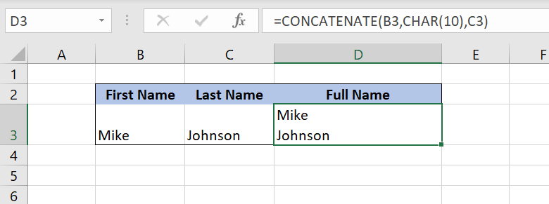
As a result, the first name is in the first row of the cell D3, while the last name is in the second row. This is also the example of using the function as a parameter of the CONCATENATE function.
Concatenate a range of cells
As we mentioned in the formula explanation, the CONCATENATE function can’t take a range of cells as a parameter. Instead, we have to select every cell from a range as a separate parameter. In the next example, we want to concatenate all the names from the range B3:B8. To do this we need to type “=CONCATENATE(“ in the formula bar, hold CTRL and click on every cell in the range. The formula looks like:
=CONCATENATE(B3,B4,B5,B6,B7,B8)

As a result, we get all the names from the range B3:B8 concatenated in the cell D3.
If you have Excel 2016 or newer, another way to do the same is to use the CONCAT function. This function takes a range as a parameter. If we want to concatenate all the values from the range B3:B8, we need to type “=CONCAT(“ in the formula bar and select the range. The formula looks like:
=CONCAT(B3:B8)
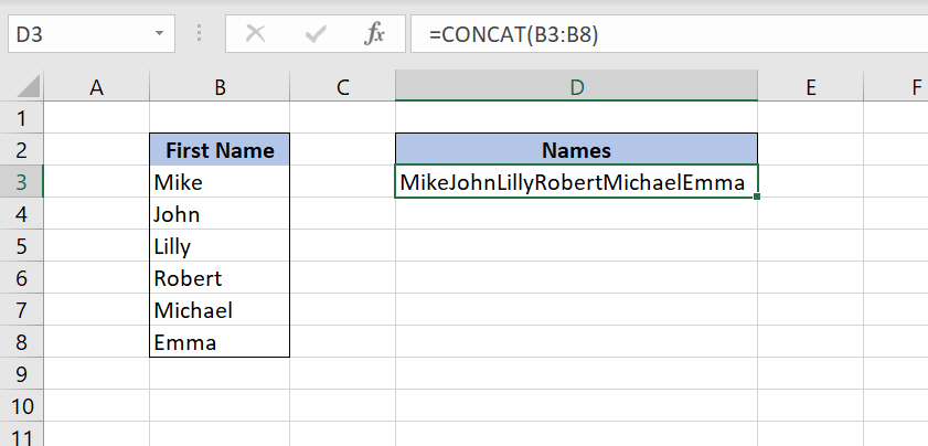
The result in the cell D3 is the same as in the previous example.
Common error when using the CONCATENATE function
The CONCATENATE function may return an error if one of the parameters is a function. In this case, if the result of the function is an error, the CONCATENATE will also return an error. Let’s explain this using an example. In the cell E3, we want to concatenate values from B3, C3 and D3, separated by spaces. The cell C3 contains #VALUE! error as a result of a function:
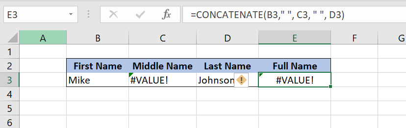
As you can see in Image 9, the result of the CONCATENATE function in the cell E3 is #VALUE! error, as the consequence of the error in C3.
In order to prevent the error when using the function as the parameter of the CONCATENATE function, we can use the IFERROR function. This function checks if a selected cell contains an error and returns a given value instead of an error. The formula is:
=CONCATENATE(B3, “ “, IFERROR(C3, “”), “ “, D3)
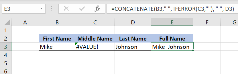
As you can see from the formula, we check the value in the cell C3 and if it’s an error, we return an empty string (“”). As a result of the formula, we get “Mike Johnson”, because the error value from the cell C3 is replaced by an empty string.
Final thoughts
All in all, the CONCATENATE function could prove very useful in many cases but if you don’t need cross-version compatibility and are using the latest (2016) version of Excel, we recommend using the CONCAT function instead. It provides added functionality and reduces the length of the function name and its arguments.