
Excel function XIRR is a financial function which returns the internal rate of return for a series of cash flows, occurring at irregular period intervals. The XIRR function includes an initial investment and net income values. This function is derived from the IRR function which does the same calculation but works only with regular (equal) periods. On the other side, the XIRR function uses irregular intervals.
In this article, we will show how to use XIRR function to calculate the internal rate of return for irregular intervals. Also, we will explain what are the possible causes of errors in the function.
Formula Syntax Explanation
The syntax of the XIRR function in Excel looks like:
=XIRR(values, dates, [guess])
The parameters of the function are:
values – a range of cells which contain cash flow values;
dates – a range of cells which contains corresponding dates for cash flow values;
guess – is an optional parameter; here we can specify our estimation of expected IRR. If this parameter is omitted, the default value is 10$.
Please note that at least one value from the value range has to be negative. This value represents a cost or an investment. All other positive values represent income from the investment. Also, dates must be sorted from the oldest to the newest and formatted properly in Excel.
Example 1 of the XIRR function
We will now look at the example to explain how the function works. Let’s first look at the data that we will use:
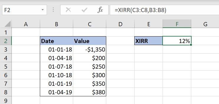
As you can see in the Image 1, in column B we have dates, while in column C we have cashflow values. As a result, we want to get the internal rate of return in the cell F2. The formula looks like:
=XIRR(C3:C8,B3:B8)
The values parameter in our formula is the range C3:C8 and the dates parameter is the range B3:B8. The final result of the function in F2 is 12% for given values and dates.
Example 2 of the XIRR function
In this example, we will see how to calculate XIRR for several periods. We will use the same example, but calculate the internal rate of return for 3 and 6 periods. Let’s see both examples:
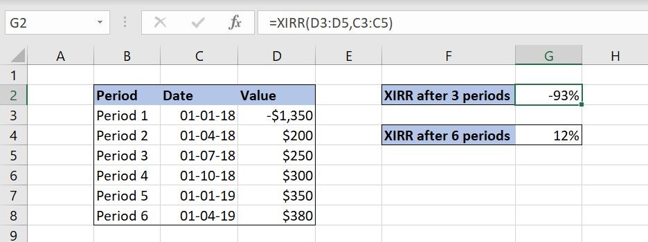
In Image 2, we want to calculate the IRR for the first 3 periods from our data set. In that case, we will select the first 3 rows from our table. Therefore, the values parameter is the range D3:D5 and the dates parameter is the range C3:C5. The result of the function in the cell G2 is -93%.
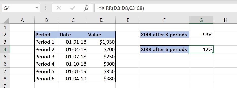
In Image 3, we want to calculate the IRR for all 6 periods. In this case, the values parameter in our formula is the range D3:D8 and the dates parameter is the range C3:C8. The final result of the function in G2 is 12%.
Common XIRR errors
Finally, we’ll look at some of the most common errors while using the XIRR function and possible causes.
#VALUE! Error
The #VALUE! Error happens if we don’t format dates appropriately and Excel can’t recognize these values as dates. Here is one example of this error:
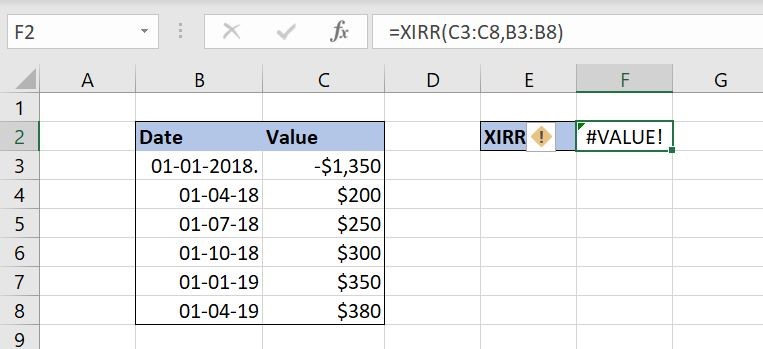
As you can see in the Image 4, the first date in column B is wrongly formatted. We added the point at the end of the date, while the correct format of the date should be dd-mm-yy, like in the other rows. As a result of the XIRR function, we got #VALUE! in the cell F2.
To reiterate, if we get the #VALUE! error, we should check the dates format and correct them.
#NUM! Error
The #NUM! Error can have multiple reasons. First, this error can occur if some of the values don’t have an appropriate date. In other words, every value must have a specified date. Let’s look at the example.
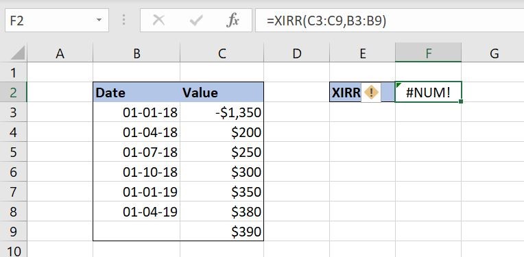
In this example, we added one more row to our range. As you can see in the Image 5, value in the cell C9 ($390) doesn’t have a corresponding date (the cell B9 is empty). As a result of the function, we get the #NUM! error in the cell F2.
Another possible cause of the #NUM! error is not providing a negative value to the function. As we stated at the beginning of the article, at least one value must be negative. This value represents the investment (cost), while all other, positive values, represent return. Here is an example of this case.
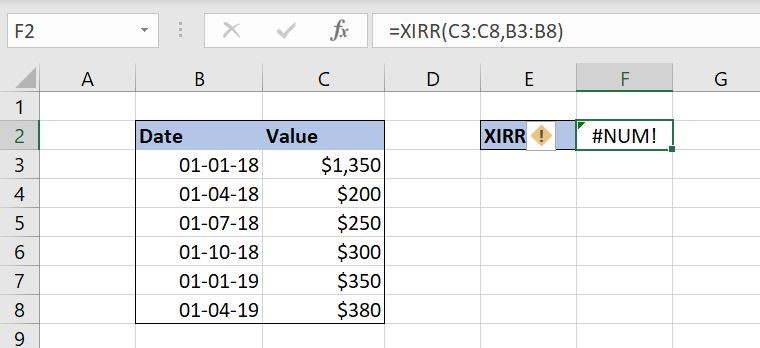
If you look at the values parameter of our function (column C), you will see that all values are positive and none of them are negative. Because of that, we got the #NUM! error in the cell F2 as a result of the XIRR function.
As we saw in the previous examples if we get #NUM! error, we should check if all the values have corresponding dates. If that is ok, we should further check if one of the values is negative.
Final Thoughts
As you can see from the examples above, the XIRR function is quite easy to understand and implement. And as with any other function, error may occur, but fixing them shouldn’t be too difficult.
Have you encountered any other XIRR errors? Let us know in the comments below!
How to use XIRR if all values with their corresponding dates are in same row?