
Conditional formatting is a very useful Excel functionality that helps us visualize data based on certain criteria. In this tutorial we will cover some of the best uses for it and show you how to create your own Conditional Formatting rules using Excel formulas.
Topics covered in this tutorial:
Creating a conditional formatting rule
Comparing values and visualizing your KPI data
Checking duplicates in two columns
Visualizing data based on multiple criteria
Marking rows that contain cells with specific characters
Creating a Conditional Formatting Rule
Let’s go through the steps needed to create a Conditional Formatting rule.
1. First, you have to select the cell, cell range or table in Excel where you want to apply Conditional Formatting
2. Find the Conditional Formatting button under tab Home -> Styles
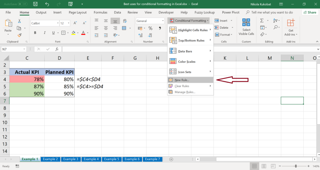
3. Click on Conditional Formatting and choose New Rule
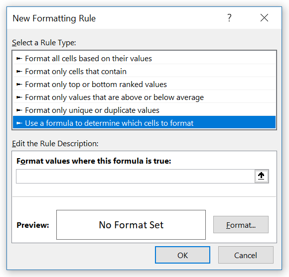
4. Choose Use a formula to determine which cells to format
5. You can create the formula rule under the section Format values where this formula is true, and specify the format under the tab Format
6. When you create the rule click OK to save it
Comparing values and visualizing your KPI data
Below is an interesting example of Conditional Formatting rules that show KPI variations from the target. To do that we will have to follow the steps from the previous point to open the New Formatting Rule window.
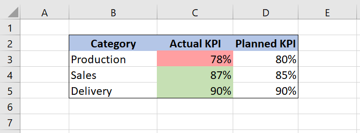
Our goal is to color the actual KPIs in red when they are below the plan and in green when they are equal or above the plan. Because of that, we will have to create two Conditional Formatting rules:
When KPI is below the plan insert =$C3<$D3 and under format select the red color.
When KPI is equal or above the plan insert =$C3>=$D3 and under format choose the green color.
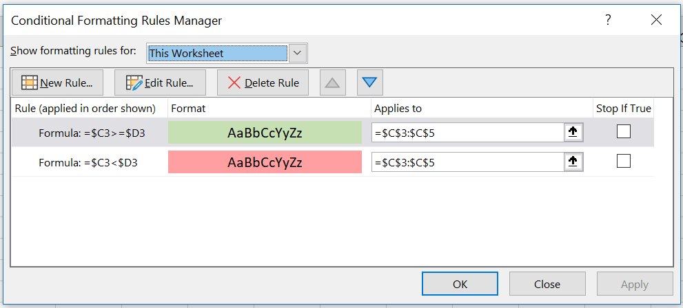
Please note that we put the absolute reference ($ sign) in front of the column in the formula. This means that you can copy the rules with the Format Painter and the columns in the rule will remain the same (C and D).
Checking for duplicates in two columns
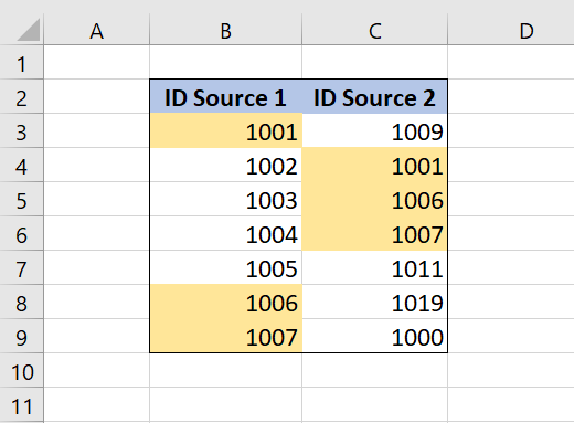
We can use Conditional Formatting to check for duplicates in two columns. Since there is no built-in Excel rule for these purposes, we will have to create our own Formula rule with Excel MATCHfunction.
MATCH function looks up the value in the table and retrieves the relative position of that value in the table. If the array is a column, the formula result will be a row number.
The parameters of the MATCH function are:
lookup_value – a value which position in an array we want to get
lookup_array – an array in which we want to find a position of a value
match_type – a type of match which will be returned. We will use 0 because we want the exact position of a value.
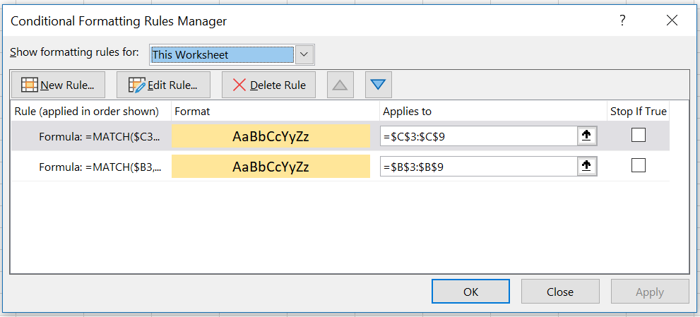
To check for duplicates in two columns we will have to create two Conditional Formatting formula rules with the MATCH function:
=MATCH($B3,$C$3:$C$9,0)>0
This first rule will check if there are values in the second column and will color them.
=MATCH($C3,$B$3:$B$9,0)>0
The second rule will do the same, but for the first column
Visualizing data based on multiple criteria
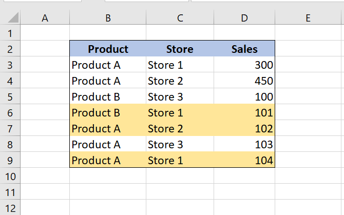
To highlight the rows based on multiple criteria, we can use formula rules in the Conditional Formatting. Let’s look in the example below where we highlighted the rows that contain Product A and have a sales value of less than 400.
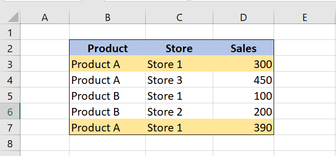
To do this, we should use the AND function and create a new Conditional Formatting rule that has the following formula:
=AND($B3=”ProductA”,$D3<400). We also need to pick a color in the format section.
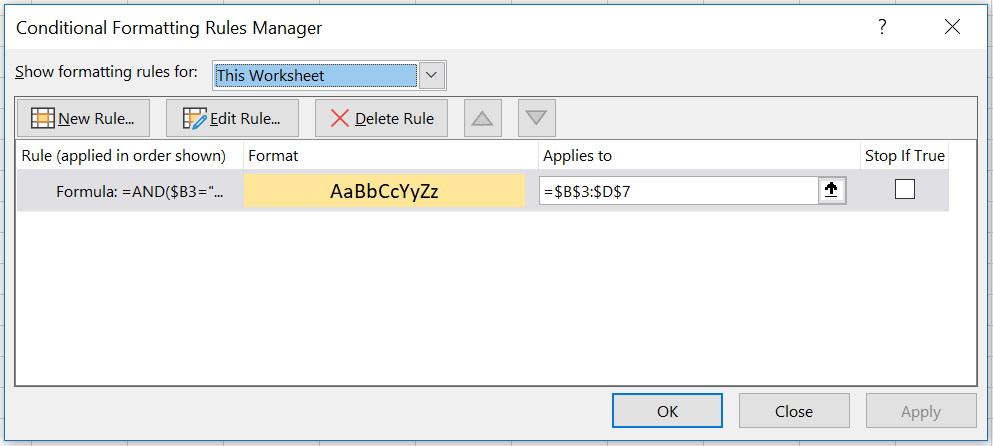
If both conditions are true, Excel will apply the Conditional Formatting rule. As we can see in the example above, 2 table rows are colored.
Let’s look at another example of multiple criteria formatting. In this case, we will use the combination of two functions: AND and OR. We want to mark the rows containing “Store 1” or “Store 2” in the column “Store” if the “Sales” value is under 200.
1. Select the table where you want to apply Conditional Formatting. In this example it’s $B$3:$D$9.
2. Create a rule based on the formula.
3. Define a formatting color in Format tab and apply this formula as shown in the example below:
=AND(OR($C3=”Store 1″,$C3=”Store 2″),$D3<200)
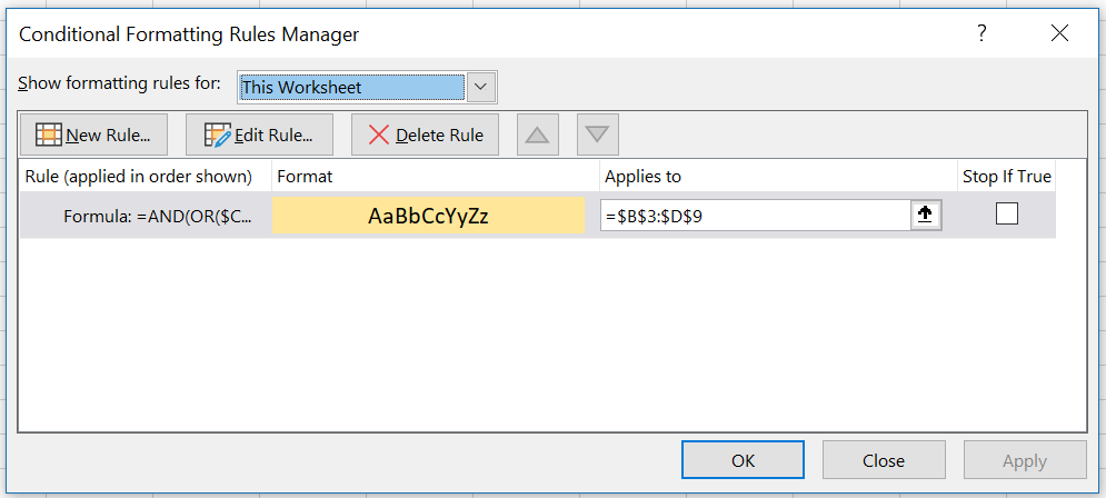
If either “Store 1” or “Store 2” is in the “Store” column and the respective “Sales” value is under 200, the row will have be formatted based on the above formula rule.
Marking rows that contain cells with specific characters
For cases where our data is not consistent (i.e a store’s name is written in multiple ways), we can use a combination of conditional formatting and the SEARCH function. With this we can color the rows that contain a specific character, phrase or word. In our example, we want to mark the rows that contain the character “a” in the column “Product”. To do this we can use the SEARCH function to find all instances of “a”. This function returns the position of one text string inside another string.
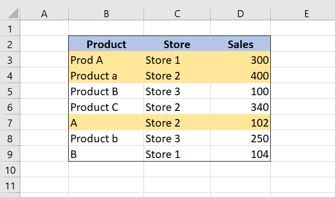
First, we have to select the table ($B$3:$D$9) and create a new formula rule:
=SEARCH(“a”,$B3)>0
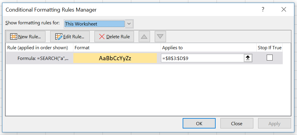
We added “>0” to the rule so that the format would only apply when the SEARCH function returns at least one instance of our string, which in this case is “a”.
Final Thoughts
As you can see there’s a lot you can do with conditional formatting and there are definitely many other uses that we haven’t covered in this tutorial. Are there any examples that you thing we should have mentioned? Let us know in the comments below!