
Excel’s VLOOKUP function is a powerful and helpful function that can help filter your data down to a desired item. It is sort of a combination of database functionality and search engine ease to refine your spreadsheet’s content to some given search item.
However, VLOOKUP for all of its powerful abilities can sometimes be frustratingly difficult to properly use. Oftentimes, this frustration is none greater than when you know that the data exists in your sheet, but you just cannot get the VLOOKUP function to work properly in returning the data. Well, worry no more because the following article provides a comprehensive approach for how to deal with the eight most common VLOOKUP errors, including how to fix them.
- The lookup value is not located in the first column of the table array to be searched.
- An exact match for your lookup is not found.
- Your table array contains duplicate values.
- You are receiving a #VALUE! Error for the lookup’s return value.
- You receive a REF! Error for the lookup’s return value.
- The lookup value is a large, floating point type of number.
- The lookup value is less than the lowest value in the table array.
- The table array reference has changed, but you have not updated the table reference.
Explanation of the VLOOKUP Formula
First, it helps to have a brief discussion about what the VLOOKUP formula is and how it works. The technical version of the VLOOKUP function is: VLOOKUP(lookup_value, table_array, col_index_num, [range_lookup]).
Translated to non-technical language, that is: VLOOKUP(the value you want to look up, the range where the value is located, the column number (reference) in the range that has the value you want returned, do you want an exact match (use 0/FALSE here) or an approximate match (use 1/TRUE here).
When should you use VLOOKUP?
In essence, you use the VLOOKUP to specify some search criteria (i.e., the lookup value) that you want to find in a specific range of cells (i.e., the table array which includes the lookup value and the value you want returned). Additionally, you specify with the VLOOKUP to look in a specific column (i.e., the column index (number)) and give me back that column’s corresponding information. Depending on whether you want that to be an exact match or not is the optional variable in the VLOOKUP formulation.
Therefore, the VLOOKUP allows you to perform a query. Think of the “V” in VLOOKUP as along the vertical row where you find the information, then give me back the corresponding information in this given column.
With that understanding of the VLOOKUP formula, the actual use of this querying tool can help provide quick and efficient results. However, when this tool is not finely tuned with the right information, errors can occur, and the following tips help recognize and solve some of the major problems found when using the VLOOKUP formula.
8 Most Common VLOOKUP Errors:
1. The lookup value is not located in the first column of the table array to be searched.
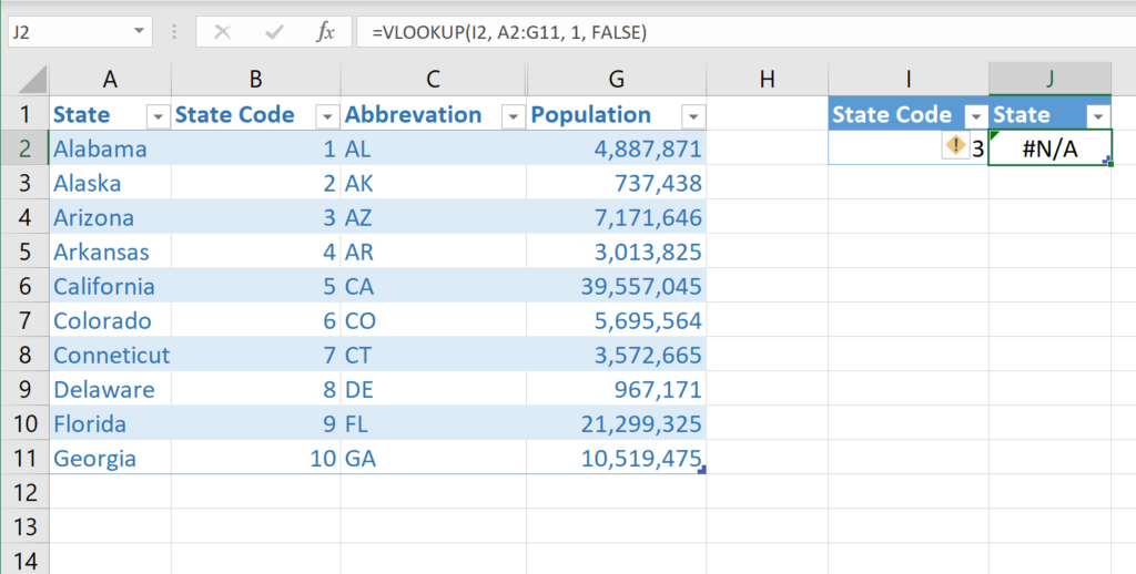
With the VLOOKUP, if you get the #N/A error, it could be that the value you are searching for is not properly specified within the VLOOKUP formula’s text. Correcting the formula and how it specifies the column where the lookup value resides can help fix this error. Make sure that within the VLOOKUP’s text, that the table array’s range has the column where the lookup value can be found or matched up to.
For example, if you specify a VLOOKUP(I2, A2:G11, 1, FALSE), this is telling Excel to look at the A2:G11 range and find the I2 value specified. When Excel finds the I2=3 value, you are then telling it to return whatever the corresponding value is in Column A. However, the I2 value resides in Column B and Excel cannot look to a preceding column in order to answer your query, so the #N/A error is returned instead.
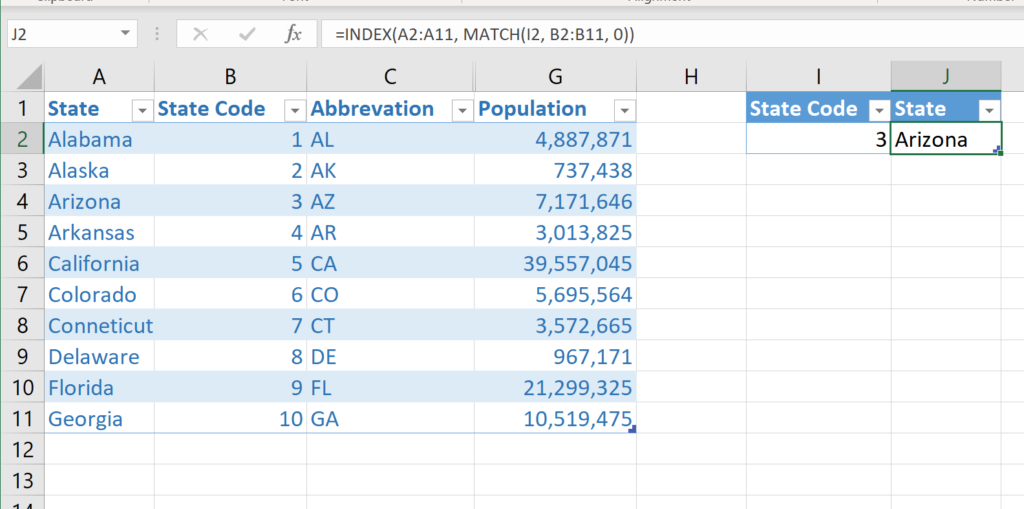
What if you can’t change the column order?
If reorganizing the VLOOKUP formula’s text and/or the columns in the range where you are specifying the search to occur are not feasible, then using the INDEX and MATCH functions may be a better alternative to the VLOOKUP in this instance. Using INDEX and MATCH combined can allow you to keep the current column order but find the appropriate match within the specified table array’s range.
2. An exact match for your lookup is not found.
If you are not receiving the desired information back from the VLOOKUP, but you know that the desired information is within the specified range, then an adjustment to the VLOOKUP function’s text could fix the problem. Errors under this topical area are usually of two types: 1) you get back the wrong information from the function or 2) the computer returns a #N/A error.
Both errors have to do with whether an exact match criterion was specified.
Remember that the VLOOKUP has the optional variable in which you can specify if you want it to find an exact match or not. Leaving this optional variable blank, or unspecified, means that VLOOKUP will assume that you want the default answer, which is TRUE = an approximate match is OK. For the function to work properly without the last variable, your data needs to be in ascending order.
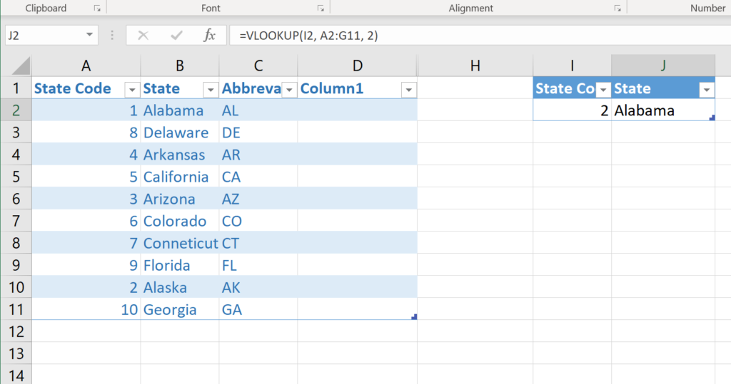
Function Returns the Wrong Information
If an approximate match is alright as part of your answer set, then the column where Excel will search for the answer should be indexed. If it is not indexed by being sorted in ascending order, then incorrect information will be returned by the formula.
In the below image, the VLOOKUP formula is being told to look for the desired value in Column B. Column B is not sorted in ascending order though, so Excel returns an incorrect match.
Formula Returns #N/A Error
If your formula is returning #N/A instead and you are sure that the desired return data does exist in the specified range, then the solution lies in making sure that the referenced cell range has the right type of data and that data is properly formatted.
Particularly, making sure that the referenced cells are free of extraneous/non-printing characters or any hidden spaces could resolve this error. Also, making sure that cell data types are correctly specified can help alleviate this problem (e.g., making sure cells that are supposed to be numbers are formatted as Number data types and not Text). You can use functions like CLEAN or TRIM to help clean up your data.
Another way to resolve the #N/A error is to specify that an exact match is desired. By making the optional variable = FALSE, you are telling the VLOOKUP that an exact match must be made. If specifying FALSE, then the data does not have to be sorted either.
The INDEX and MATCH functions are another way to resolve errors for these reasons as well. See INDEX and MATCH references for additional details.
3. Your table array contains duplicate values.
VLOOKUP is designed to only return one value and that value will be the first one that it encounters where the lookup value is found. If you have duplicate values that match the lookup value, then you may not get the desired, correct return value. There are two things that you can do in this situation: 1) clear out duplicate data, if feasible and 2) use a PivotTable instead if you need the duplicate data to stay in your range.
Clearing Out Duplicates
To easily rid your data range of duplicate values, select the data range where the VLOOKUP will be looking, and then, go to the Data tab and select Remove Duplicates. This will remove any duplicates that exist in the data range that you have highlighted. Thereafter, the VLOOKUP should be able to properly find and match the desired values.
Using a PivotTable
Instead, if you need the data to stay as-is, with the duplicates in place, then VLOOKUP will not work for you. A PivotTable will be a better and more robust way to get at the data you desire. Think of PivotTables as allowing you to do the same VLOOKUP and then some. The querying power of the PivotTable will be able to sort through your duplicates and still return meaningful information.
4. You are receiving a #VALUE! Error for the lookup’s return value.
If you have worked with VLOOKUP frequently enough, chances are that you have encountered the #VALUE! error before. The #VALUE! error occurs in two instances: 1) the lookup value exceeds 255 characters and 2) the column specified within the function where to look for results is less than 1.
The Lookup Value Exceeds 255 Characters
If the lookup value exceeds 255 characters, you should look to shorten this value, if feasible. 255 characters is the maximum length allowed for this string. If shortening the value is not feasible, then the INDEX and MATCH combination could be used to do your querying instead.
Specified Column is Less Than 1
Where the #VALUE! error occurs due to the VLOOKUP containing a column index (i.e., col_index_num) that is less than 1, the resolution is to re-evaluate the table array range and specify a different column index number. The minimum number allowed for this value is 1, and 1 references the column where the lookup value can be found. Thus, the column index would have to be some column to the right of column 1, and hence, a number greater than 1 also.
5. You receive a #REF! Error for the lookup’s return value.
If you are seeing #REF! error, that means that the VLOOKUP’s column index argument (i.e., col_index_num) needs to be adjusted. This error appears if the column that you are referencing is not part of the range that you are specifying. To correct this, make sure that the column index you are specifying lies within the VLOOKUP’s table array range.
6. The lookup value is a large, floating point type of number.
If the cells you are searching have time values or are large decimal numbers, VLOOKUP cannot handle more than 5 decimal points. Thus, you get a #N/A error. Time is stored as a floating decimal point value.
The solution to this problem is to use the ROUND function to truncate the table array’s cell data down to 5 decimal points and this will alleviate this error.
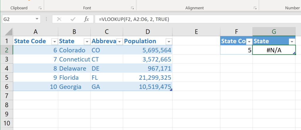
7. The lookup value is less than the lowest value in the table array.
You can also get the #N/A error when your specified lookup value is less than the values in the column that you are instructing the VLOOKUP to look in for that initial matching. The optional range lookup for an exact match argument has to also be set to TRUE (or left blank within the VLOOKUP) in order for this error to occur.
For example, if your lookup value is 5 and all the values in the column to search are greater than 5, with the exact match argument set to TRUE, you will get this #N/A error.
To fix this problem, either adjust the lookup value to match the range of numeric values in the column to search, or if that is not feasible, use the INDEX and MATCH functions to get the data you desire instead.
8. The table array reference has changed, but you have not updated the table reference.
If for any reason you make modifications to the table array after you have already written the VLOOKUP formula, then Excel may return the #N/A error. Things that alter the size and dimension of the table array (e.g., adding or deleting a column, increasing the number of rows, moving around the original order of columns, etc.) could render VLOOKUP unable to find your specific lookup value.
To solve this, go back to the VLOOKUP function and check to make sure that all of its arguments properly align with the new size and dimension of the table array.
Conclusion
The VLOOKUP function is a popular and powerful tool within Excel that can deliver pinpoint accuracy of searches throughout your spreadsheet(s). However, VLOOKUP can deliver a lot of frustrating errors and misinformation if not properly configured with its various arguments.
Take time to note the error you are receiving, and then, use this guide to help diagnose and resolve the problem. Remember, sometimes your ultimate resolution may involve using additional Excel functionality, like a PivotTable, the INDEX and MATCH functions, CLEAN, ROUND and TRIM may all assist in getting the results you desire.